Klaus Haller, 13.5.2020
Click here to download the tutorial as a pdf file – or scroll down to read it online…
1. Aim of this Computer Vision Introduction Tutorial

Deep Learning, Analytics, Computer Vision – these are some of today’s hot topics in the IT industry. These are key technologies for innovation. Universities and big tech companies put high efforts in research and engineering in these areas. However, even individual developers can enrich their applications with such artificial intelligence and computer vision technology if they on existing technologies, tools, and libraries.
This short tutorial explains you one way to achieve this. We use Python and Jupyter Notebook running on Amazon SageMaker to “implement” image classification based on available, pretrained neural networks within one to two hours. In other words: You will learn that you do not need any research, no Ph.D., and not two years and a big team to incorporate such features in your applications.
The first half of the tutorial is about navigating the AWS web console, whereas the second part covers the code to get your first images classified.
2. Amazon SageMaker / Amazon Sage Maker Studio
SageMaker is Amazon’s solution for machine learning. It comes with one big benefit if you start learning computer vision with SageMaker: You do not have to do any installations on your local laptop. When you have your AWS login, it takes you less than five minutes and you can start with development work. And it is free, at least for the first two months and if you use it moderately, i.e., you stay away from expensive AMIs or extra options.
To continue, you need an AWS account and you have to be signed in to your AWS account. Alternatively, you have to have a local Jupyter Notebook installation on your computer. In this case, you can continue with section 3 “Understanding Juypter Notebook”.
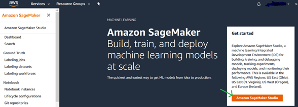
xxWhen you are signed in to your AWS account and you are in the AWS services page, you type in “SageMaker” and select and click on the service.

Then, you click on “Amazon SageMaker Studio”, which is Amazon’s development environment.
Next, you create a new user for SageMaker Studio. Therefore, click on “Add user”.

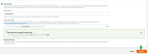
Select “Quick start, add a user name, and select “Create new role”.

A mask shows up for creating an IAM role. If you are in a test environment, just accept by clicking on “Create Role”.
Now you can create the SageMakerStudio environment by clicking on “Submit”.
A couple of times, I had issues with the submit button. I could click it, but there was no reaction. In such a case, you are most probably a person with some experience using AWS. You might want to choose the “standard setup” option and choose an existing VPC or subnet.
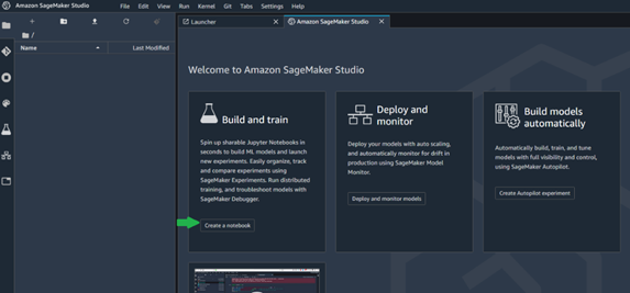
A little bit later (it might take a while), you see the following page and you can select “Open Studio”.

Now, click the “Create a notebook” button.
You get to the following screen:
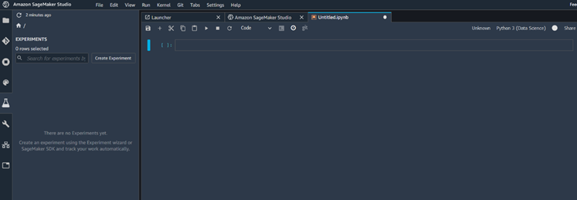
Congratulations. You are now ready to go! The next section will give you a brief introduction in Juypter Notebook and how to use it as a development environment.
3. Understanding Juypter Notebook
Jupyter Notebook is a development environment used by many data scientists. Compared to your typical Java Eclipse IDE, there are important differences:
- You work interactively like you might know it from interpreted languages. You write some lines of code to download data, query your data, or to train a machine learning model – and you see the result immediately.
- Jupyter Notebook is like a paper notebook when it comes to documenting. You write down the code and add comments to it immediately. In contrast to commenting your code in Java, you can make it look nicer, it feels more natural, and it really helps that you work interactively. You write what you want to achieve as a comment, then you write the code. Then you continue with the next comment, followed by code again.
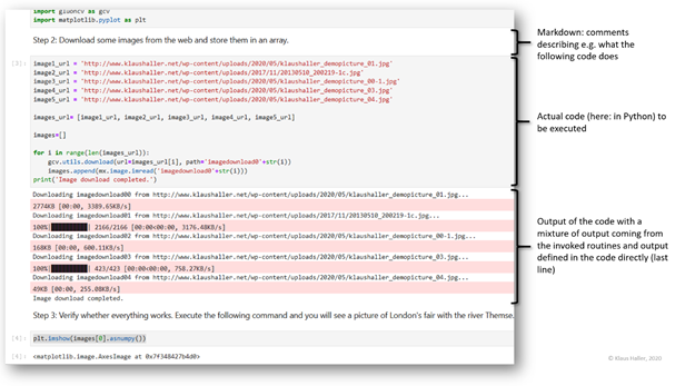
Figure 1 provides an example, a screenshot showing part of the code of this tutorial. The screenshot shows the second step where we download the images from the web and store them in an array for later processing. On the top, we see a cell with comments or text. This is called “markdown”. It is followed by a cell with actual code. We define variables, then download the images in a for-loop, and write to the console that we are finished. Down there, we see the output that was written to the console when we executed the code cell.
4. Implementing Image Classification in Python
It is straight forward to implement an image classification using Python. We do not need our own training data and we do not have to train a neural network. We just use existing models available for download from the web. You can either copy & paste the input for the cells from the tutorial or type the code in by yourself.
Input the following to the cell on the Juypter Notebook.
**
** This script demonstrates image classification using Python 3 and Gluon-CV.
** (c) Klaus Haller, 13.5.2020
**
Then, change the cell type from “Code” to “Raw” …

… and press Shit+Return.
We are ready for the the first step. We begin with a comment:
Step 1: Load the librariesChange the cell type to “Markdown” and press Shift+Return.
We have to download and install some libraries:
pip install mxnet gluoncv matplotlibOnce you press Shift+Return, you see an output similar to the following (it might look different if you run it the first time):
Requirement already satisfied: mxnet in /opt/conda/lib/python3.7/site-packages (1.6.0)
Requirement already satisfied: gluoncv in /opt/conda/lib/python3.7/site-packages (0.7.0)
Requirement already satisfied: matplotlib in /opt/conda/lib/python3.7/site-packages (3.1.3)
Requirement already satisfied: numpy<2.0.0,>1.16.0 in /opt/conda/lib/python3.7/site-packages (from mxnet) (1.18.1)
[…]
Requirement already satisfied: setuptools in /opt/conda/lib/python3.7/site-packages (from kiwisolver>=1.0.1->matplotlib) (45.2.0.post20200210)
Note: you may need to restart the kernel to use updated packages.
Now, we import the libraries to our notebook:
import mxnet as mx
import gluoncv as gcv
import matplotlib.pyplot as plt
As for all other code cells, we have to press Shift+Return to execute the commands (in the following, I will not mention this again).
Aim of the next step, the second step, is to download the pictures we are using and loading them to an array. We write the following short text in a markdown cell:
Step 2: Download some images from the web and store them in an array.We continue with the actual code we want to execute:
image1_url = 'http://www.klaushaller.net/wp-content/uploads/2020/05/klaushaller_demopicture_01.jpg'
image2_url = 'http://www.klaushaller.net/wp-content/uploads/2017/11/20130510_200219-1c.jpg'
image3_url = 'http://www.klaushaller.net/wp-content/uploads/2020/05/klaushaller_demopicture_00-1.jpg'
image4_url = 'http://www.klaushaller.net/wp-content/uploads/2020/05/klaushaller_demopicture_03.jpg'
image5_url = 'http://www.klaushaller.net/wp-content/uploads/2020/05/klaushaller_demopicture_04.jpg'

images_url= [image1_url, image2_url, image3_url, image4_url, image5_url]

images=[]

for i in range(len(images_url)):
    gcv.utils.download(url=images_url[i], path='imagedownload0'+str(i))
    images.append(mx.image.imread('imagedownload0'+str(i)))
print('Image download completed.')
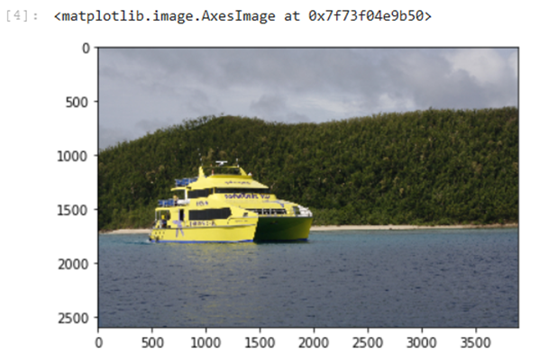
You can verify whether everything worked perfect by submitting the following command:
plt.imshow(images[0].asnumpy())You should see a yellow boat on the sea with a small beach and forest in the background.
Step 3 is about preparing the images so that they can be classified (dealing with different sizes, brightness etc.). We start again with a markdown cell documenting what we do:
Step 3: Prepare the images for object identificationThe actual code follows here:
images_prepared=[]
for i in range(len(images)):
  images_prepared.append(gcv.data.transforms.presets.imagenet.transform_eval(images[i]))
In the following 4th step, we install a pretrained neural network. This means, it is a neural for which all training is completed. It is ready to classify our sample pictures.
Step 4: Initialize pretrained neural and classify imagesThe code for step 4:
pretrainedNN = gcv.model_zoo.get_model('densenet201', pretrained=True)
top3classes=[]
for i in range(len(images_prepared)):
    top3classes.append(mx.nd.topk(mx.nd.softmax(pretrainedNN(images_prepared[i])), k=3)[0])
The following code shows the images and the three most likely classifications for the image. To prevent misunderstandings: The neural network classifies (hopefully) the most dominant object on the image, though looking at the second or third most likely class can be an indication what else is on the picture.
print('Picture 1')
plt.imshow(images[0].asnumpy())
for i in range(3):
    index=top3classes[0][i].astype('int').asscalar()
    label=pretrainedNN.classes[index]
    print('#',i+1, 'Detected object: ', label)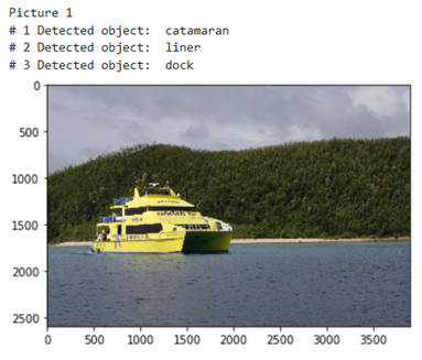
Obviously, the first classification is perfect.
Now we have a look at the second image and how it is classified by the neural network:
print('Picture 2')
plt.imshow(images[1].asnumpy())
for i in range(3):
    index=top3classes[1][i].astype('int').asscalar()
    label=pretrainedNN.classes[index]
    print('#',i+1, 'Detected object: ',label)
print('Picture 3')
plt.imshow(images[2].asnumpy())
for i in range(3):
    index=top3classes[2][i].astype('int').asscalar()
    label=pretrainedNN.classes[index]
    print('#',i+1, 'Detected object: ',label)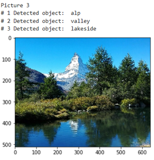
This picture does not have one dominant object, but various ones – the Matterhorn mountain in the Alpes, some trees in the middle, and a lake in the foreground. Again, the suggested classes – at least alp and lakeside – make sense.
Now the fourth picture.
print('Picture 4')
plt.imshow(images[3].asnumpy())
for i in range(3):
    index=top3classes[3][i].astype('int').asscalar()
    label=pretrainedNN.classes[index]
    print('#',i+1, 'Detected object: ',label)
This picture contains a bottle of sparkling wine and a champagne flute as larger objects, plus a table, a plastic chair, and a tree in the background. Again, the algorithm works well with suggesting a wine bottle. The alternative, beer bottle, is also not bad.
The neural network has the goal to classify the image, aka the main object, correctly. It does not aim to identify the second or third most important or biggest object on the image. Also, the exact objects – sparkling wine bottle and champagne flute – were not trained. Thus, the neural network cannot identify them as such.
The last picture is one with me.
print('Picture 5')
plt.imshow(images[4].asnumpy())
for i in range(3):
    index=top3classes[4][i].astype('int').asscalar()
    label=pretrainedNN.classes[index]
    print('#',i+1, 'Detected object: ',label)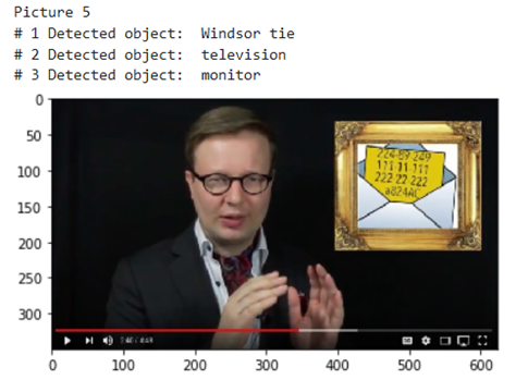
Obviously, this pretrained neural network does not identify a human plus some illustration in the background well. However, that is nothing the neural network was trained for – and this is to make you aware that pretrained neural networks have also their limitations and cannot solve everything.
To conclude: It takes an hour or two to classify pictures using pretrained neural network. This has implications for projects in companies. It makes no sense to start a project with checking for existing pretrained neural networks before embarking in time-intense software engineering and neural network endeavors. The pretrained models do not beat a human, but in many cases, they might be enough to start your journey of using images to generate new knowledge and new insights for your company.